Structural variant visualization

JBrowse 2 has several complementary views for exploring structural variants (SVs). SV calls are loaded as variant tracks (VCF/BCF); reads as alignments tracks (BAM/CRAM). A typical workflow starts with the SV inspector — a combined variant table and whole-genome circular overview — to triage candidates, then uses the alignments displays to examine read-level evidence at each breakpoint. This guide covers the SV-focused interpretation of those tools; see the alignments track guide for general alignments features.

For an end-to-end walkthrough that loads a real cancer dataset (HG008 tumor and normal PacBio HiFi reads plus the C-GIAB benchmark SV/CNV call sets) and exercises each of the views described below, see Cancer Genome in a Bottle (SVs).

SV signals in the alignments track

The standard alignments track gives you several SV-relevant signals without requiring any extra steps:

• Soft clipping — reads that extend past a breakpoint have their overhanging bases soft-clipped; enabling Show soft clipping (Track menu → Pileup settings → Show...) makes these bases visible at breakpoint edges
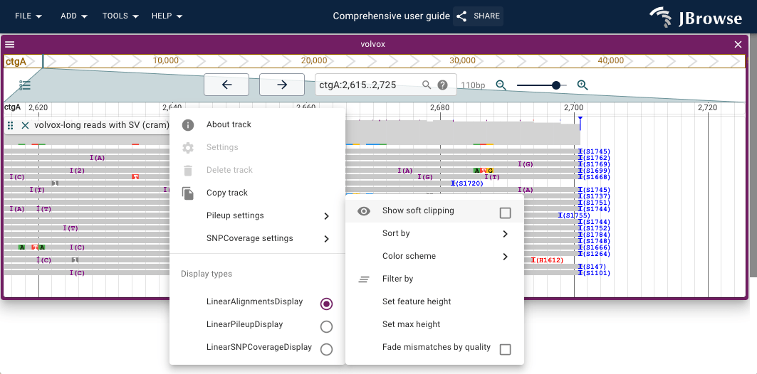
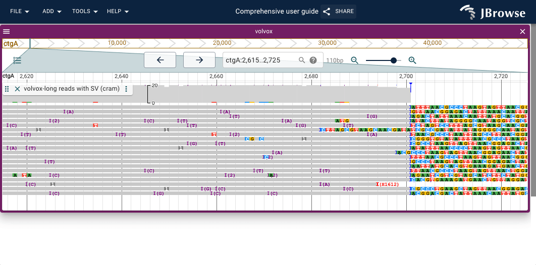
• Insertion/clipping indicators — a purple triangle marks positions where more than 30% of reads carry an insertion; blue/red triangles mark clipping; larger purple rectangles appear for insertions >10 bp
• Color by pair orientation — abnormally oriented pairs produce characteristic colors described in the table below
• Color by insert size — pairs with unexpectedly large or small inserts are highlighted

For descriptions of these features in general use, see the alignments track guide.

Pair orientation color scheme

JBrowse uses the same color scheme as IGV — see the IGV paired-end alignments guide for background. Enable via Track menu → Pileup settings → Color by... → Pair orientation. The library type (fr, rf, or ff) can be changed via Pileup settings → Orientation type; the default is fr (Illumina). SOLiD-style pair orientations are not supported. The table below assumes fr:

Orientation	Color	Description
LR (→ ←, normal proper pair)	light grey	concordant
RL (← →, mates pointing away from each other)	green	abnormal orientation
LL (→ →, both mates forward strand)	teal	abnormal orientation
RR (← ←, both mates reverse strand)	dark blue	abnormal orientation

An inverted duplication with characteristic orientation patterns: RL pairs (green) and LL/RR pairs (teal/dark blue) at the structural variant boundaries.

Insert size color scheme

In the pileup (Track menu → Pileup settings → Color by... → Insert size), reads are colored by a continuous HSL gradient based on insert size; reads with mates on a different chromosome are dark grey.

In the read arc and linked reads displays (Track menu → Color scheme), the Insert size ± 3σ option uses threshold-based coloring:

Pattern	Color	Notes
Insert > mean + 3σ (larger than expected)	red	suggests a deletion spanning the pair
Insert < mean − 3σ (smaller than expected)	pink	suggests an insertion between the pair
Mate on a different chromosome	purple	suggests an inter-chromosomal event

Insert size ± 3σ and orientation combines both signals and is often the most informative setting for a general SV scan.

SV-type signatures

The patterns below describe what each SV type typically looks like in the alignments track. They are clues, not proof — final interpretation still requires judgment. The DRAGEN SV IGV tutorial is a useful companion reference.

Deletion

• Soft-clipped reads at two nearby positions mark the breakpoint edges
• A coverage drop between those positions is a classic deletion signal; heterozygous deletions typically show only a ~50% reduction rather than a complete drop
• Paired reads flanking the gap colored red (larger insert than expected) suggest a deletion spanning the pair
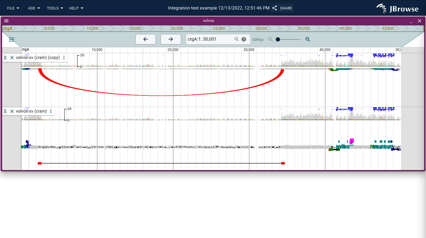
• In the read arc display, unusually long arcs point to a deletion

Insertion

• Soft-clipped reads at a single site suggest an insertion; with Show soft clipping enabled, the inserted bases become visible on each side
• When the insertion is large enough that pairs flank it, those pairs colored pink (smaller insert on reference) suggest an insertion between them
• For insertions larger than the sequenced fragment size, mates may become unmapped; long reads are needed to fully span the event
• A purple insertion indicator triangle suggests an insertion when >30% of reads carry one at that position

Inversion

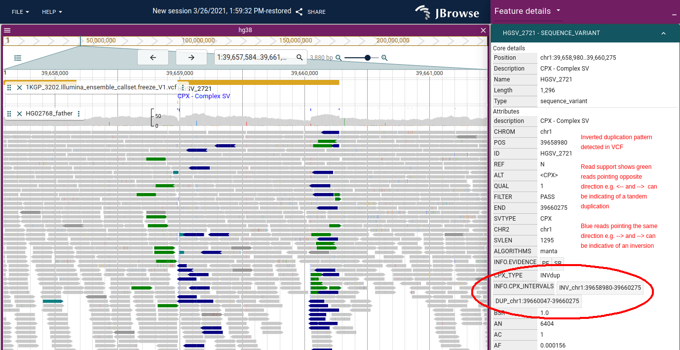
• LL (teal) and RR (dark blue) read pairs at a boundary suggest an inversion — normally LR-oriented reads become same-direction across the junction
• If you're zoomed into the inverted region itself, interior reads may look concordant
• Soft-clipped reads appear at both breakpoints, sometimes with short homology sequences visible in the clipped bases

Tandem duplication

• RL (green) read pairs suggest a tandem duplication: reads appear to point away from each other when the duplicated segment is joined back to its origin
• Elevated coverage over the duplicated region is another supporting signal
• In the read arc display, arcs pointing backward (upstream) across a junction point to a tandem duplication

Translocation / inter-chromosomal fusion

• In the read arc and linked reads displays, reads with mates on a different chromosome are colored purple; in the pileup they appear dark grey
• A cluster of such reads at a locus marks one end of a translocation; open the breakpoint split view from the feature details to see both ends at once

Read arc display

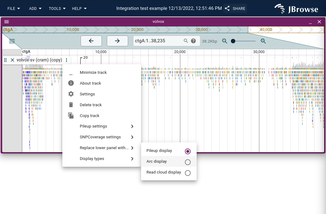
The read arc display renders bezier curves between the two ends of a paired-end read or split alignment, making long-range connections immediately obvious. Enable via Track menu → Display types → Read arc display (or Replace lower panel with... to show arcs alongside the coverage and pileup panels).

Menu item for selecting the 'Read arc display'.

Inter-chromosomal connections appear as vertical lines at the view edge. Track menu → Color scheme provides insert size, orientation, or combined coloring.

The read arc display showing a deletion with Illumina paired-end reads and Nanopore ultra-long reads on HG002.

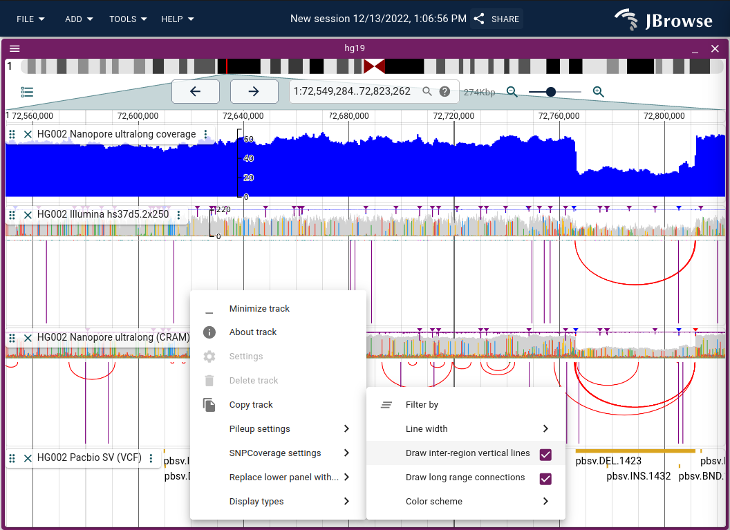
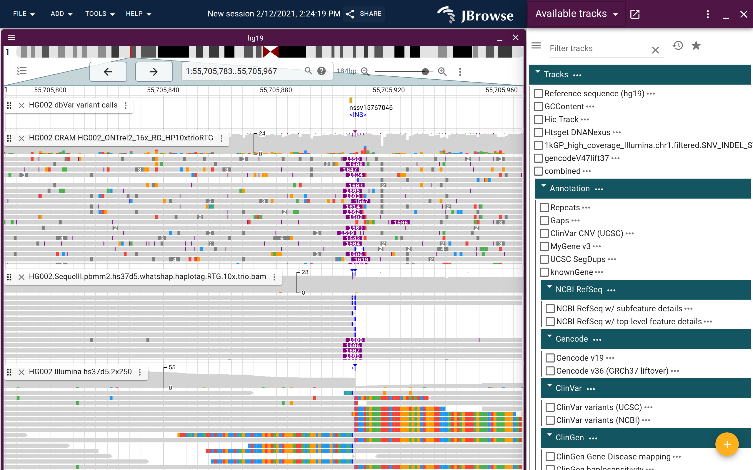
Live demo — HG002 deletion with Nanopore and Illumina reads in arc display

Linked reads display

The linked reads display draws paired-end reads and supplementary alignments on the same row connected by a line, and stratifies rows by the log-scaled distance between read ends. This makes it easy to count how many reads span a breakpoint and to see their orientation at a glance. Chains with supplementary alignments are connected by an orange line.

Enable via Track menu → Display types → Linked reads display (or Replace lower panel with... to keep the coverage and pileup panels).

The read arc display and linked reads display shown together for the same dataset.

Live demo — inversion example in linked reads mode

Track menu → Edit filters lets you show or hide proper pairs and singletons. Track menu → Color scheme provides insert size, orientation, or combined coloring.

Inspecting individual reads

Right-clicking any read opens a context menu with two single-read inspection options:

• Linear read vs ref — opens a synteny-style split view showing how that read aligns to the reference, with the read sequence on one panel and the reference on the other
• Dotplot of read vs ref — opens a dotplot of the read against the reference, which can reveal complex rearrangements as diagonal segments

Both are most useful on long reads where a single read spans a breakpoint.

A ~500bp insertion from a breast cancer cell line (SKBR3) PacBio read shown using 'Linear read vs ref'. The lower panel shows the synteny-style alignment.

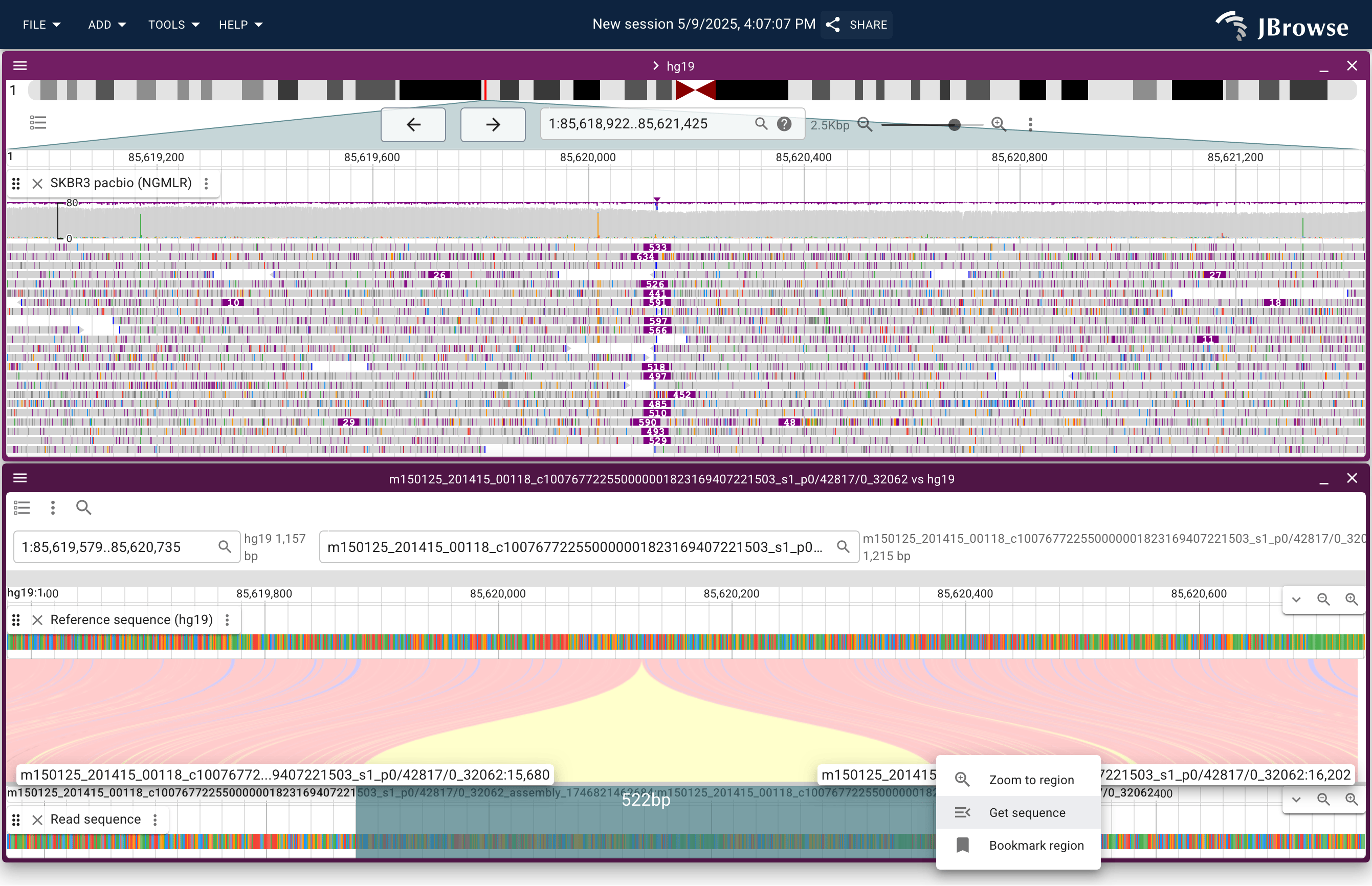
Live demo — SKBR3 PacBio read vs reference insertion

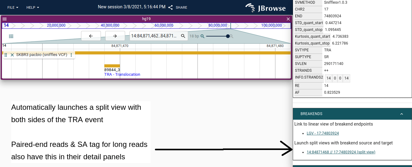
Breakpoint split view

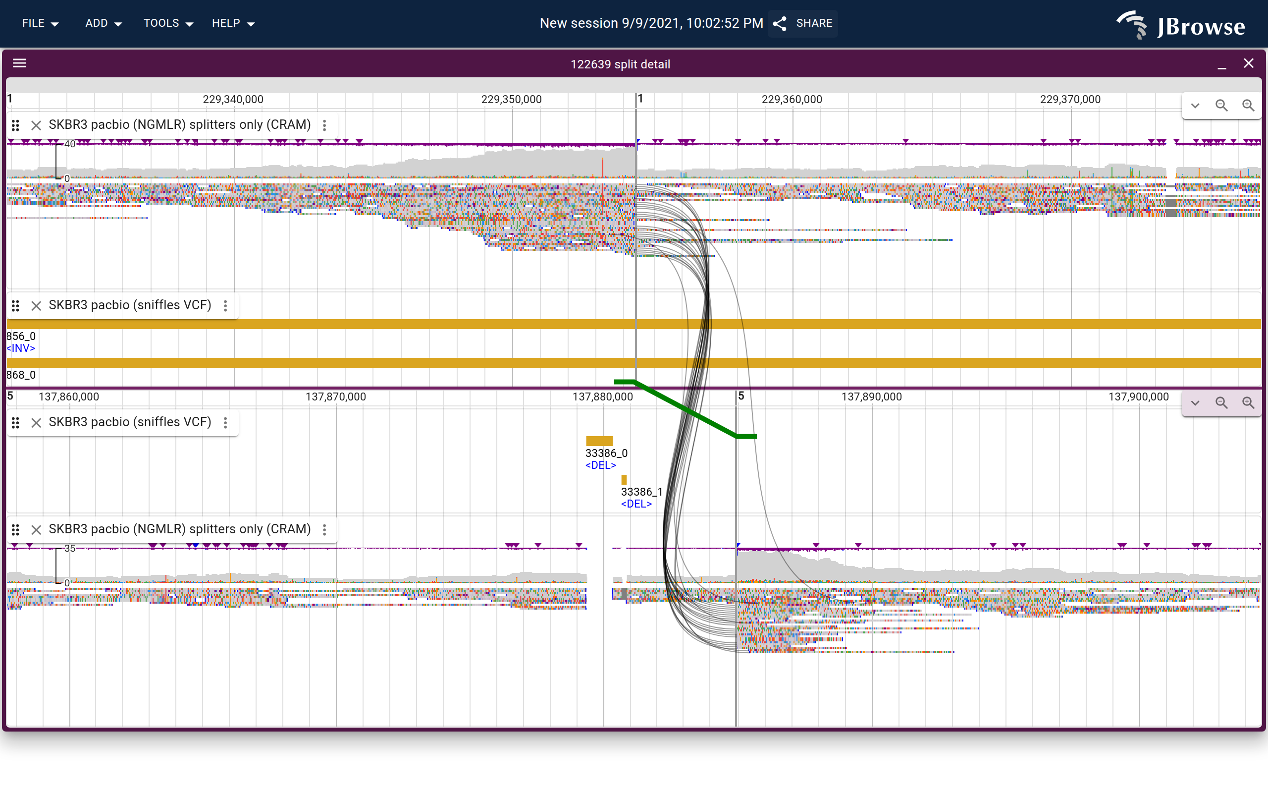
The breakpoint split view opens two synchronized panels side-by-side, each centered on one breakpoint locus. Splines connect supporting reads across both panels, and the variant call is drawn as a colored line with feet indicating directionality.

Breakpoint split view for an interchromosomal translocation. Black splines connect supporting reads; the green line with feet is the variant call.

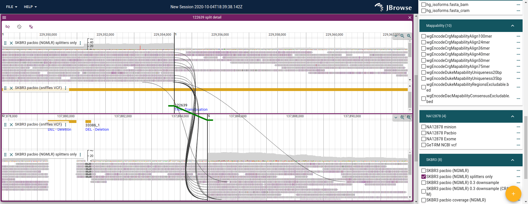
Live demo — SKBR3 interchromosomal translocation in breakpoint split view

The header bar (added in v3.7.0) accepts location searches directly in either panel.

Launching the breakpoint split view

• From the SV inspector — click a feature in the circular overview or the triangle dropdown on any table row. See the SV inspector guide.
• From variant feature details — click a BND or TRA variant in a variant track; the feature details panel has a button to open the split view, automatically loading any open alignment tracks.
• From alignment feature details — click any read with a supplementary alignment; the feature details panel includes an option to open the split view centered on that read and its supplementary partner.

The feature details panel for a BND/TRA variant has a link to open the breakpoint split view.

The view also supports multi-hop events where a single read has multiple supplementary alignments, connecting more than two breakpoints simultaneously.

Live demo — multi-hop split read connection in breakpoint split view

Phasing heterozygous SVs

For heterozygous SVs, confirming that supporting reads come from a single haplotype is strong evidence for the call. If your BAM/CRAM has been haplotagged (e.g., with WhatsHap or HiPhase), reads carry an HP tag identifying the haplotype.

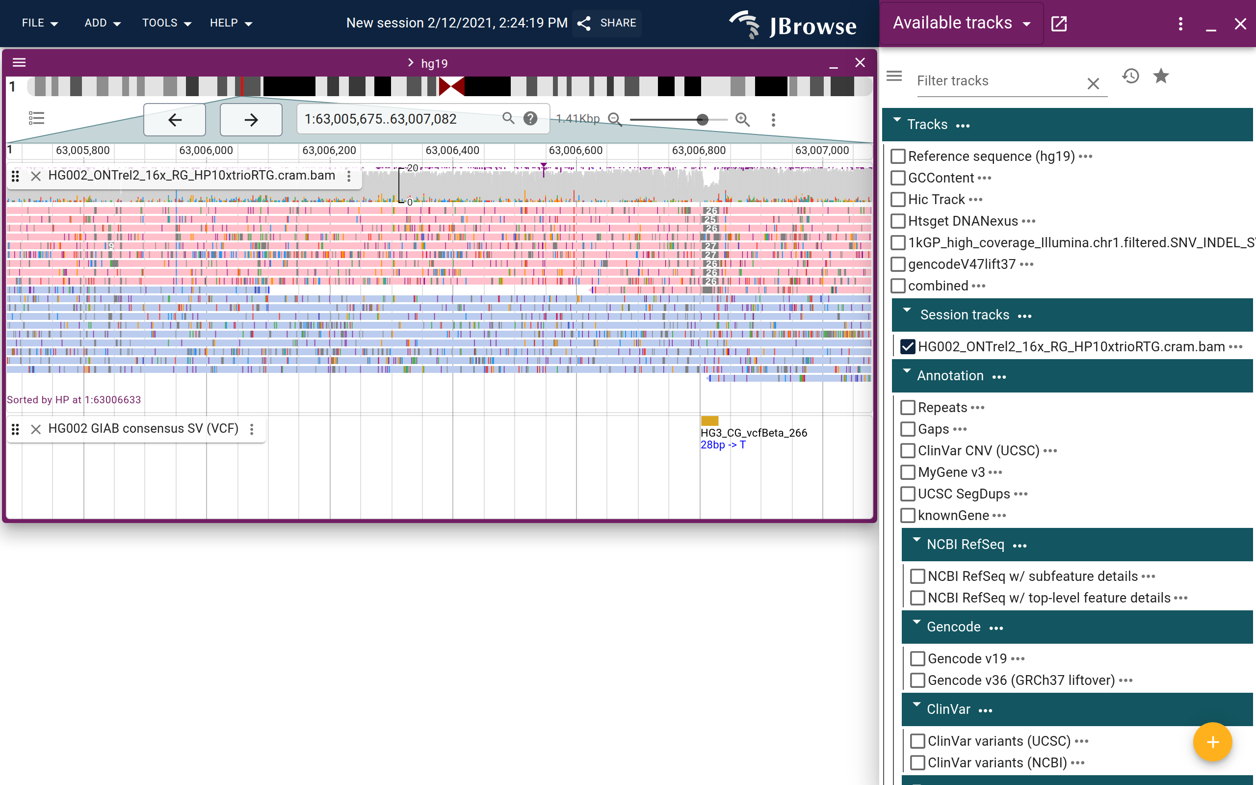
Sort and color by HP via Track menu → Pileup settings → Sort by → Tag → HP and Color by → Tag → HP. Reads from each haplotype cluster together, making it easy to see whether an SV is present on one or both haplotypes.

Step-by-step guide showing how to sort and color by haplotype with the HP tag.

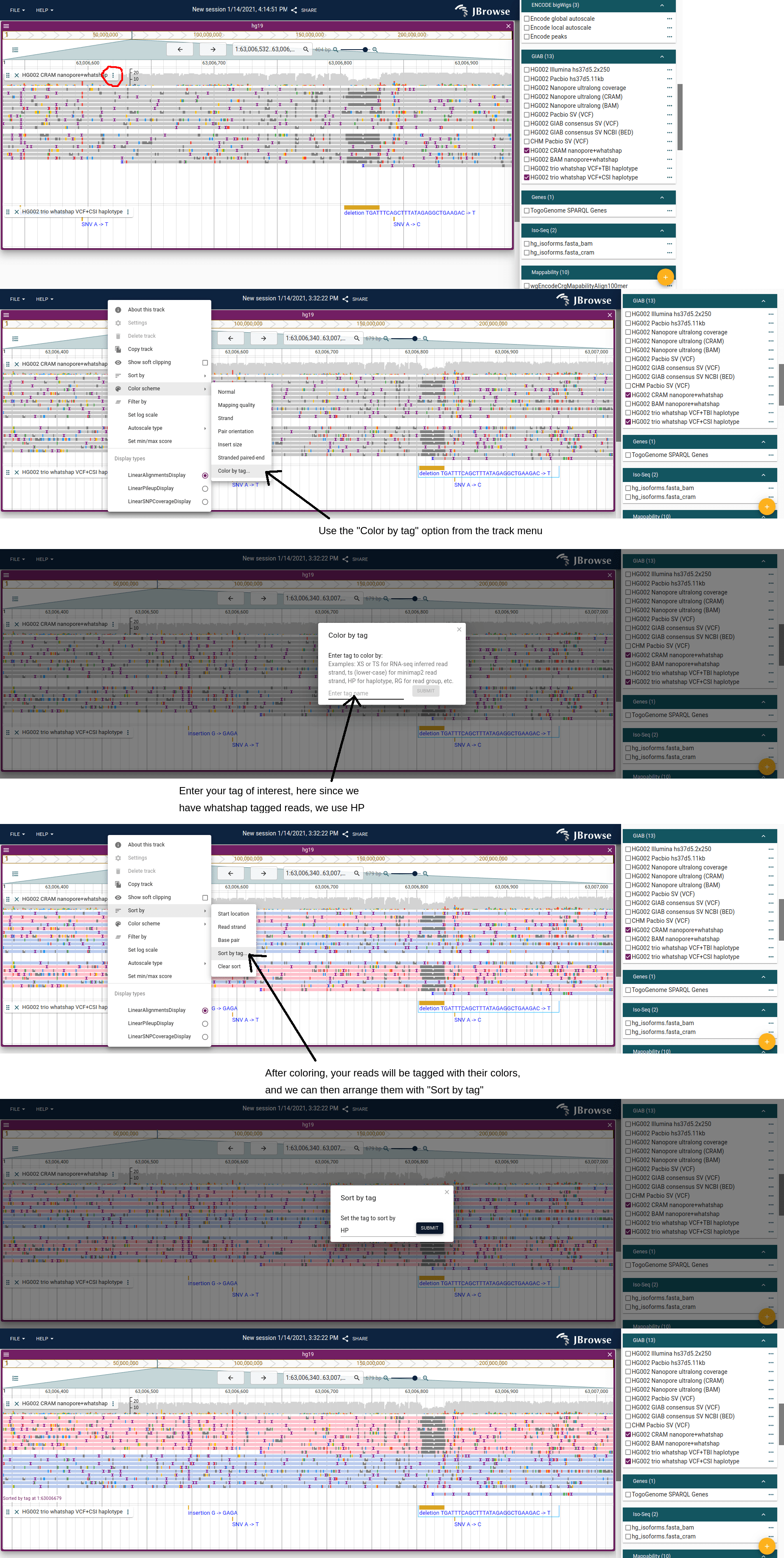
Live demo — heterozygous small deletion in GIAB colored and sorted by HP tag

Track menu → Group by → Tag → HP will split the track into separate sub-tracks per haplotype for an even clearer visual separation. Note that group by spawns new track instances dynamically, so sort and color is generally faster for initial exploration.

See the alignments track guide for more on sorting, coloring, and filtering by tag.

Working with large SVs

Loading a very large genomic region will trigger an error because JBrowse declines to fetch hundreds of megabytes at once. For large or inter-chromosomal SVs, a better approach is:

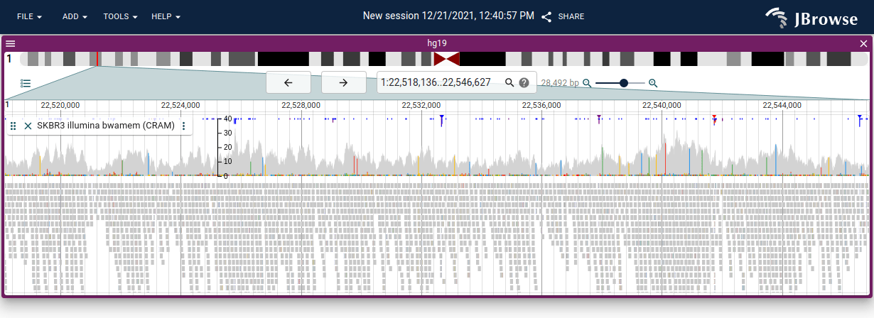
• Use a bigWig coverage track (or a multi-quantitative track for tumor vs normal comparison) instead of a full alignments track when surveying the region — it loads at any scale and makes copy-number changes immediately visible
• Load the SV call set as a variant track for a compact overview of all calls; clicking a feature navigates directly to it
• Open the breakpoint split view to inspect the breakpoint loci themselves — each panel shows only a local window around one end of the SV, so the inter-breakpoint distance doesn't matter
• Use the SV inspector for whole-genome triage before drilling into individual calls

COLO829 melanoma tumor (red) and matched normal (blue) whole-genome coverage as a multi-quantitative bigWig track. Copy-number changes are visible at chromosome scale without loading any reads.

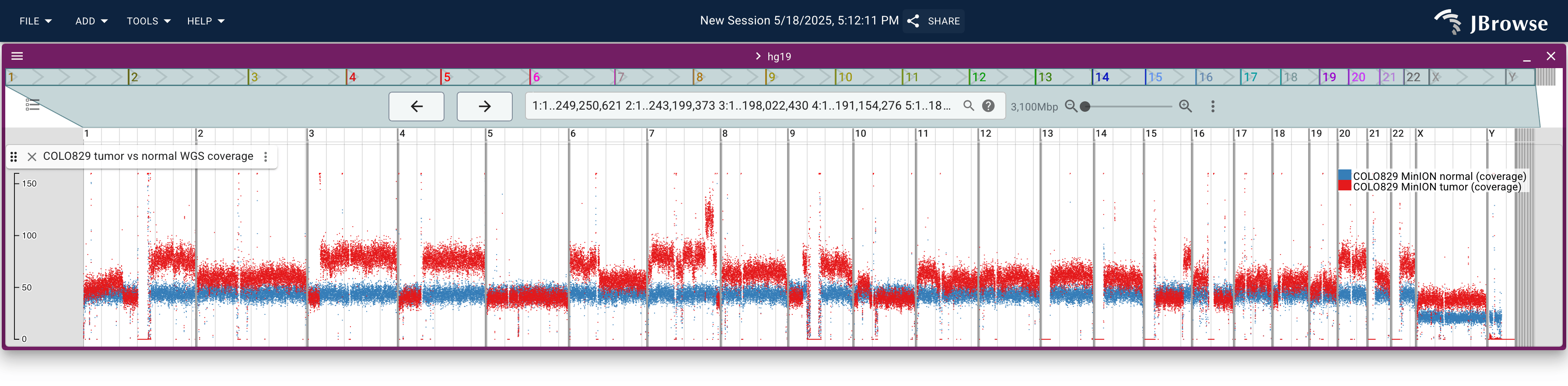
Live demo — COLO829 tumor vs normal whole-genome coverage

Whole-genome assembly comparison

When a de novo assembly of the sample is available — for example, a phased tumor assembly from PacBio HiFi or ONT data — aligning it back to the reference with a tool like minimap2 and loading the resulting PAF as a synteny track gives a chromosome-scale view of rearrangements that read-level displays cannot. Complex events like chromosomal fusions appear as off-diagonal blocks in the dotplot view, and clicking and dragging over a region in the dotplot can launch a base-level linear synteny view with the same alignment.

This is particularly effective on cancer samples, where the derived genome often differs structurally from the reference in ways that are hard to read off the alignment track. The C-GIAB tutorial walks through this workflow end-to-end with the HG008 phased tumor assembly.

Summary

Display / setting	How to enable	Best for
Pileup (default)	Default lower panel	Base-level detail, individual reads
Color by pair orientation	Pileup settings → Color by...	Abnormal orientation patterns (RL/LL/RR)
Color by insert size	Pileup settings → Color by...	Insert size anomalies (pileup, continuous gradient)
Read arc display	Track menu → Display types	Overview of long-range connections
Linked reads display	Track menu → Display types	Counting discordant pairs, orientation per read
Linear read vs ref	Right-click on any read	Complex alignment of a single long read
Breakpoint split view	Feature details or SV inspector	Side-by-side inspection of both breakpoint loci
Sort/color by HP tag	Pileup settings → Sort by / Color by → Tag	Confirming heterozygous SVs on one haplotype
Dotplot view	Launch from start screen	Chromosome-scale rearrangements (de novo assembly)
Linear synteny view	Launch from dotplot selection	Base-level alignment between two genomes

Limitations

• Read-level displays require zooming in: the pileup, arc, and linked reads displays only render when the view is zoomed in enough to load individual reads; very large SVs can't be spanned in a single pileup view
• Paired-end evidence is fragment-size limited: for insertions larger than the sequenced fragment, paired-end evidence disappears; long reads are required to fully resolve the inserted sequence
• Repetitive regions: SVs in segmental duplications or repeats produce noisy, ambiguous signals; soft-clipped reads and orientation anomalies are common artefacts in these regions
• Short-read orientation coloring assumes fr (Illumina) by default; change via Track menu → Pileup settings → Orientation type for rf or ff libraries. SOLiD-style orientations are not supported.