Alignments track
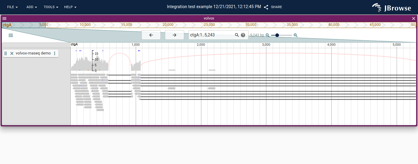
The alignments track combines a pileup and a coverage visualization.
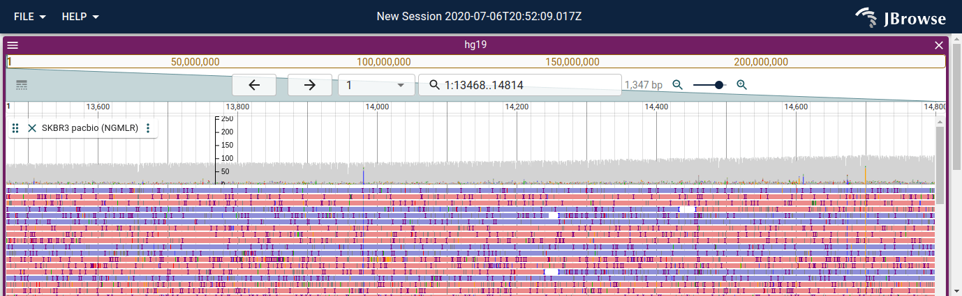
Pileup visualization
The pileup (lower panel) shows reads as boxes positioned on the genome.
By default, forward-strand reads are red; reverse-strand reads are blue.
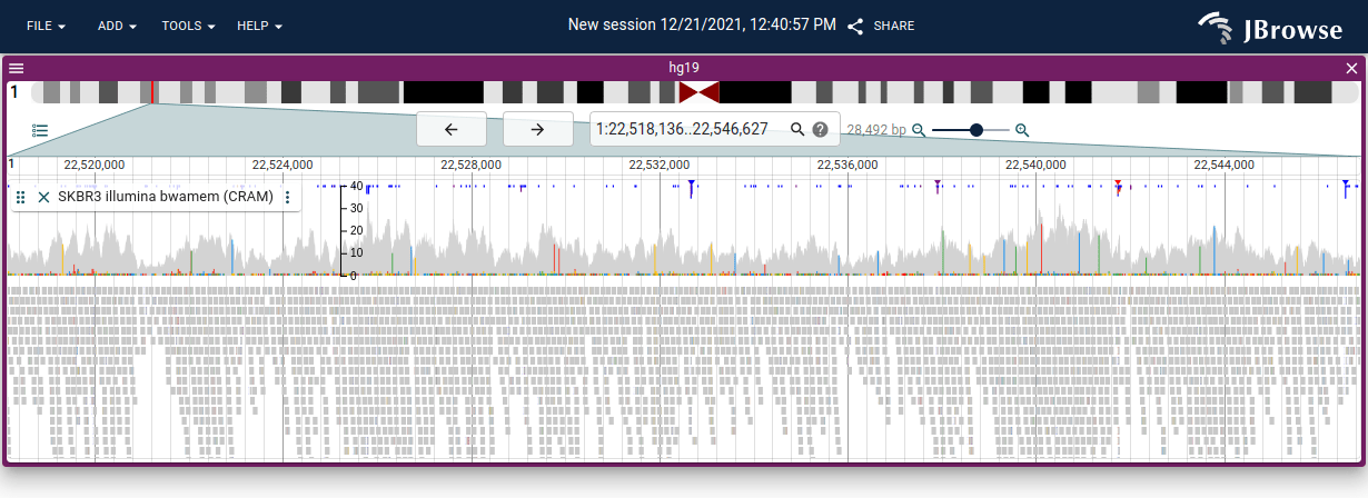
Coverage visualization
The coverage track shows depth-of-coverage at each position and highlights mismatches with colored boxes proportional to their frequency — if 50% of reads have a T where the reference has A, half the histogram height is colored.
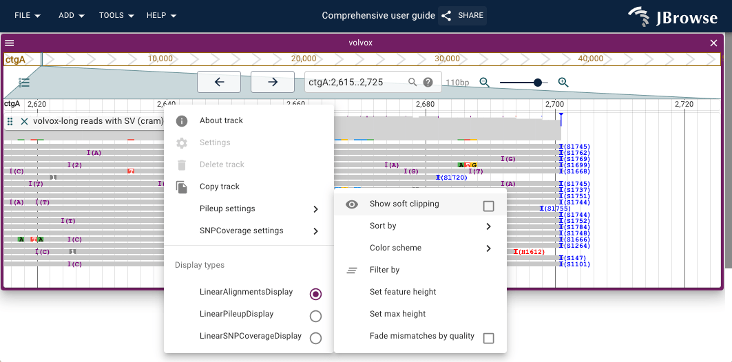
Show soft clipping
Aligners clip terminal bases that cannot be incorporated into an alignment: hard clipping discards them from the BAM record; soft clipping retains them in the BAM sequence (marked 'S' in the CIGAR) but excludes them from the alignment. JBrowse does not render soft-clipped bases by default, but enabling "Show soft clipping" (Pileup settings menu) can reveal signal around structural variants and difficult mappability regions.
Sort by options
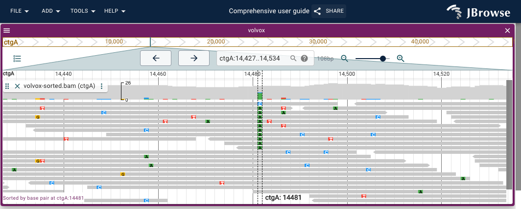
The alignments track can be configured to sort reads by a specific attribute at the center line.
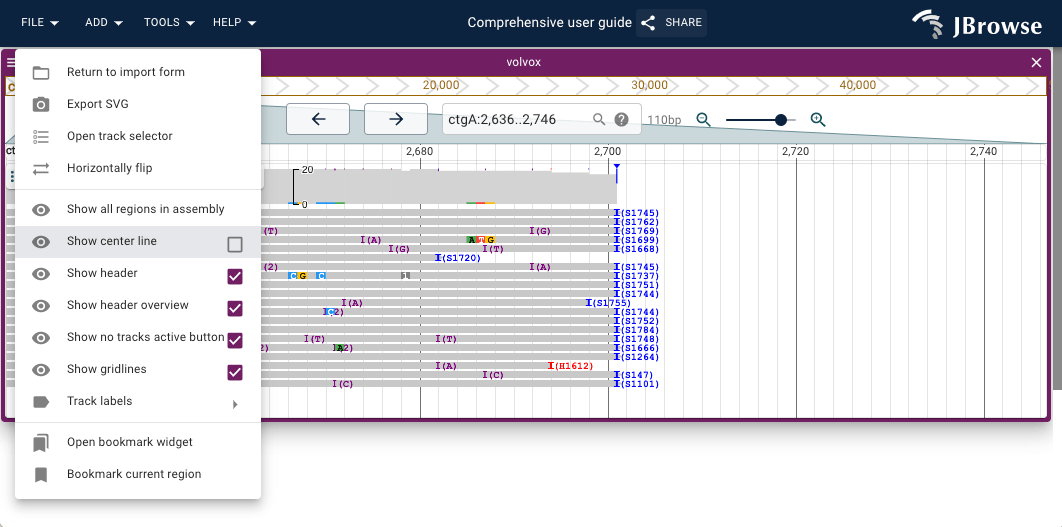
Showing the center line
- Open the hamburger menu in the top left of the linear genome view
- Select "Show center line"
The sort is performed using properties of the read, or the exact base pair underlying the center line.
Sorting by base pair
Sorts the pileup by the base each read has at the center line position. To enable:
- Open the track menu using the vertical '...' in the track label
- Select
Pileup settings→Sort by→Base pair
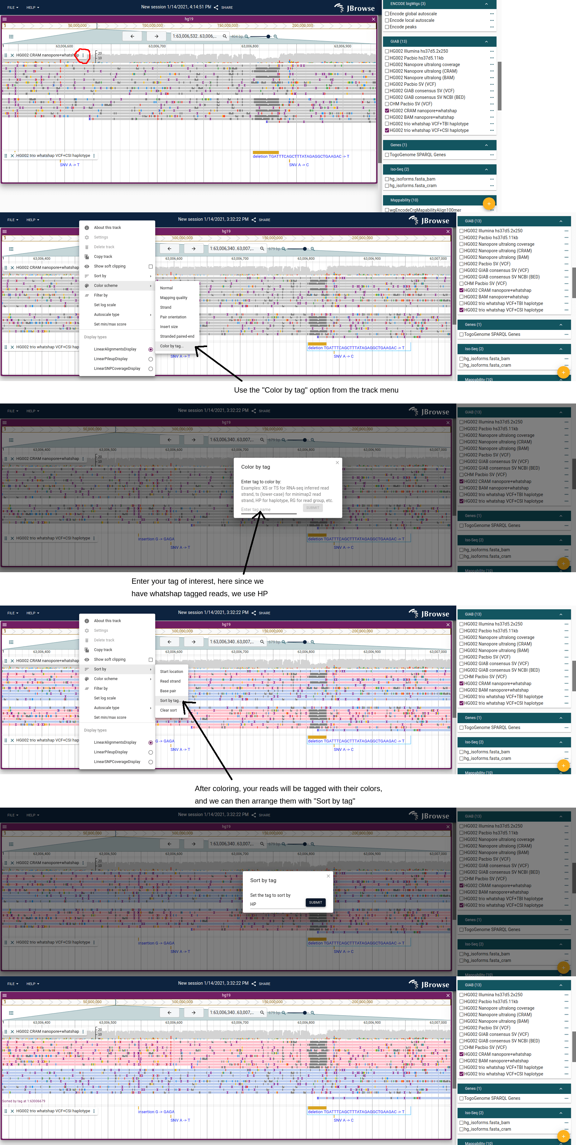
Sort, color and filter by tag
The guide below shows how to color and sort reads by the HP tag:
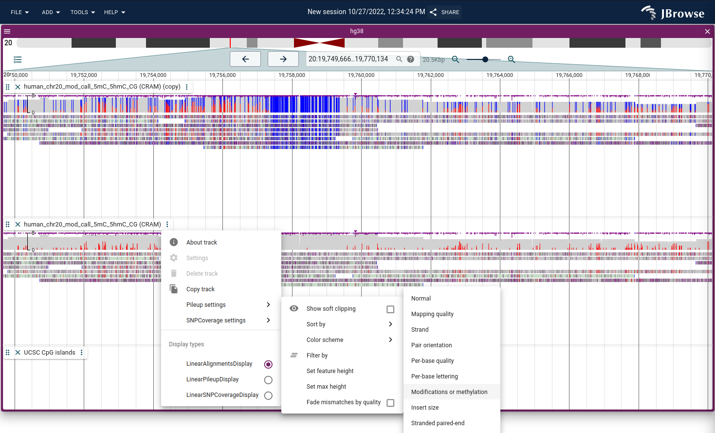
Color by modifications/methylation
The alignments track can color DNA/RNA modifications using the MM tag in BAM/CRAM files. It uses two modes:
- All modifications - draws the modifications as they are
- Methylation mode - draws both unmodified and modified CpGs (unmodified positions are not indicated by the MM tag and this mode considers the sequence context)
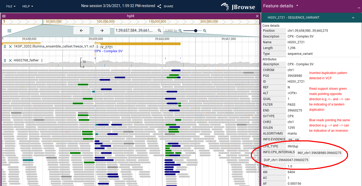
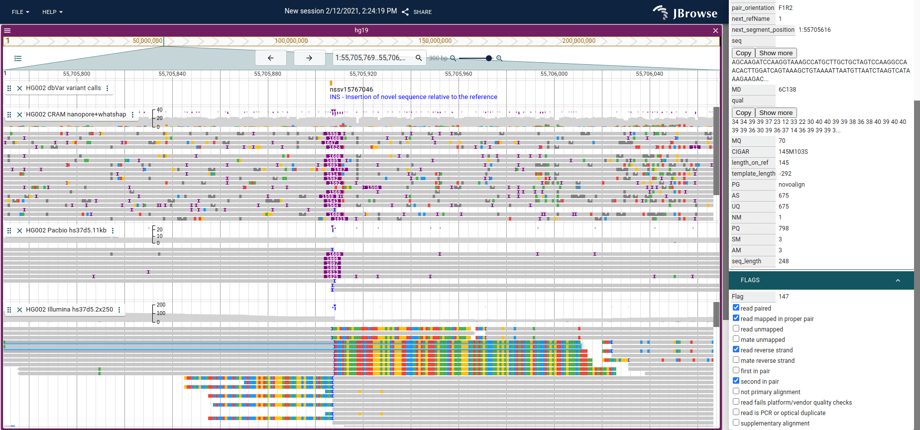
Color by orientation
JBrowse uses the same color scheme as IGV for coloring by pair orientation. These pair orientations can be used to reveal complex patterns of structural variation. For a full breakdown of what each color indicates and how to interpret each SV type, see the structural variant visualization guide.
Sashimi-style arcs
Spliced alignments (N in the CIGAR string) are drawn with sashimi-style arcs. If reads carry an XS tag, arcs reflect the strand of the alignment.
Disable via the track menu (vertical "..." next to track label) → SNPCoverage settings → uncheck "Draw arcs".
Insertion and clipping indicators
An inverted histogram of insertion and clipping counts is drawn above the pileup; positions where >30% of reads carry an event are marked with a colored triangle.
Insertions >10bp are marked with a larger purple rectangle. This signal is more prominent in long-read data, which can span larger insertions.
Disable via the track menu (vertical "..." next to track label) → SNPCoverage settings → uncheck "Draw insertion/clipping indicators" and "Draw insertion/clipping counts".
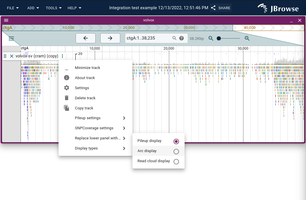
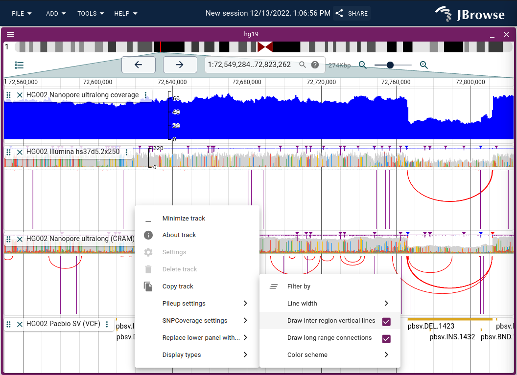
Using the "Read arc display"
The read arc display renders bezier curves between paired-end or split-read ends, making long-range connections visible for detecting SVs and misassemblies.
Enable via Track menu → Display types → Read arc display (or "Replace lower panel with..." to show arcs alongside coverage).
Dragging the track height repacks the arcs to fit, allowing dense displays with multiple tracks. Inter-chromosomal connections appear as vertical lines; off-screen interactions as larger arcs. Both can be disabled via the track menu.
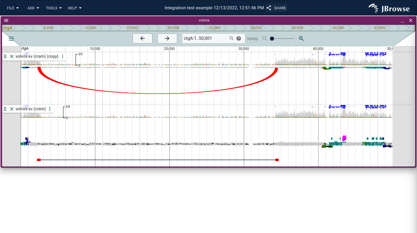
Live demo — HG002 deletion with Nanopore and Illumina reads in arc display
Using the "Linked reads display"
The linked reads display connects paired-end reads and split alignments as rows stratified by log-scaled distance between ends. Dragging the track height repacks reads into the available space.
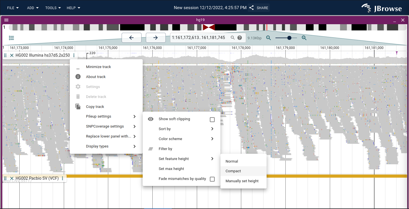
Compacting the view of alignments tracks
Enable compact display via Track menu → Pileup settings → Set feature height → Compact.