PAG 33 (2026) JBrowse setup and exploration

Introduction

This tutorial was written for the JBrowse workshop at PAG 33. As this workshop was aimed at attendees with a wide range of experience with JBrowse, it contains both introductions to general JBrowse functionality as well as some deep dives into more specialized features. We hope everyone can find something of interest in this tutorial.

This tutorial is aimed at users of JBrowse who already have access to a JBrowse instance, whether from the JBrowse 2 genome hubs, JBrowse pages on other websites, or JBrowse desktop. For information on setting up a JBrowse instance, please see our separate tutorial on that topic at PAG 33.

If you are following this tutorial after PAG 33, please note that the UI of current versions of JBrowse may differ slightly from those shown in the screenshots here.

JBrowse UI overview

Let's get started with JBrowse by opening up a JBrowse page configured with a genome of interest. For this tutorial, we'll use the mm10 mouse genome. Please use this link: https://jbrowse.org/code/jb2/main/?config=/ucsc/mm10/config.json.

Note that usually we'd access this from the JBrowse 2 genome hubs page at https://genomes.jbrowse.org/, using the JBrowse link on the mm10 mouse genome under the "Main genome browsers" section. However, we're going to be there are a couple of unreleased features that make this tutorial run a bit more smoothly, so the link above uses our latest unreleased version.

Here is what you should see when that page loads.

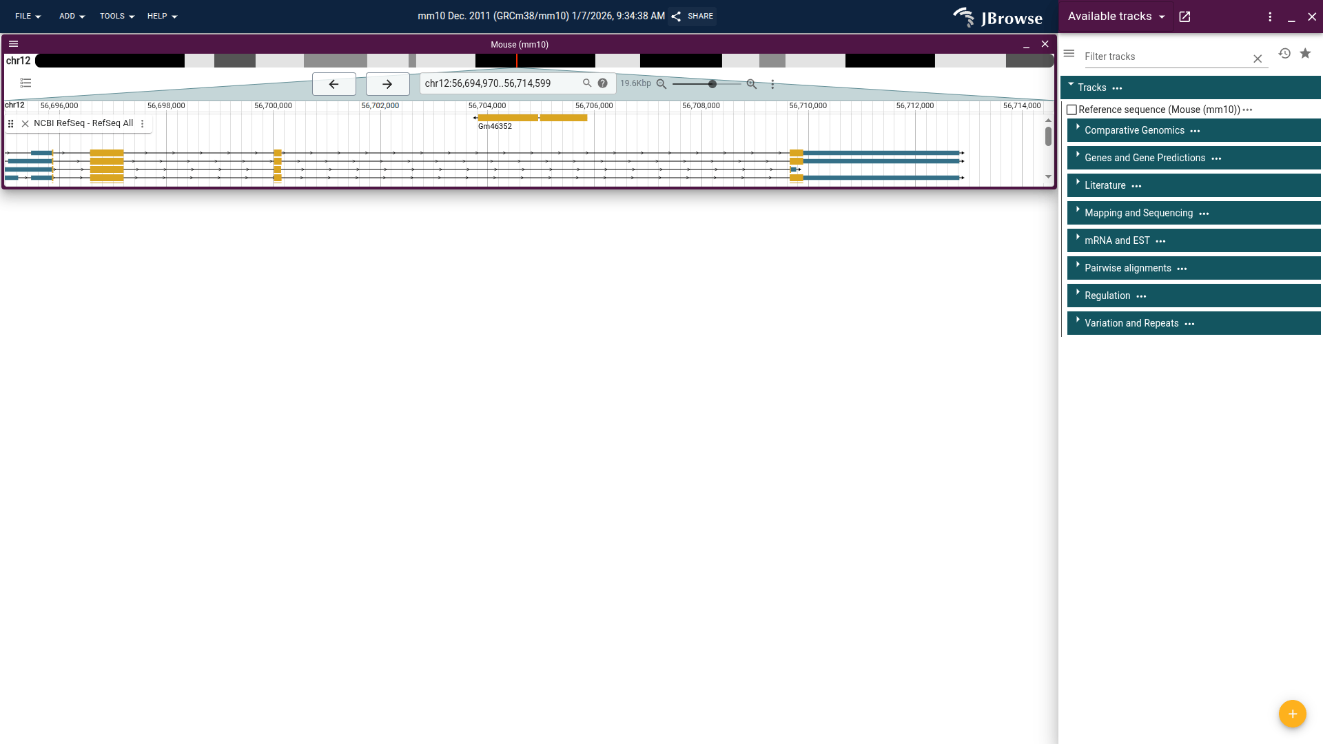
On the left you see the browser is showing the mouse genome open to a location on chromosome 12. The very top bar has menus for various actions, as well as the default name for this session and a "Share" button, which we'll explore more later.

The next area on the left is what is called a "view," open to a location on chromosome 12. This view has an overview at the top to show the currently displayed location on the chromosome, as well as some navigation controls. There is one track open in this view, "NCBI RefSeq - RefSeq All," which shows RefSeq gene annotations. If you click on the "Genes and Gene Predictions" section, it will expand to show all the available tracks in that section. You can see the filled in checkbox next to the track that is already open.

Go ahead and explore the page by trying out the different navigation buttons, opening new tracks, and hovering over or clicking on the visualizations inside the tracks. For more information on the many controls and options available in JBrowse, please see the user guide.

To illustrate an important feature of JBrowse 2, let's open a new view. From the "Add" menu at the top of the page, choose "Linear genome view." A new view will appear where you can choose an assembly (we only have one available, but some JBrowse instances will have many) and a location.

Enter "Pax9" in the location box and click "Open." The new view will now be open to the same location as we saw when we first loaded the page. We'll just use a single view for the rest of this tutorial, but having multiple views available, as well as views of different types, is a core JBrowse feature. You can see examples of some of these views on the JBrowse gallery page. For now, though, go ahead and close one of the two open views.

Adding tracks

The JBrowse 2 Genome Hubs come with a lot of useful tracks already configured, but with JBrowse you aren't limited to the existing tracks. Let's say we have our own data for the m10 mouse genome that we want to visualize. We can add that data as our own track.

For some sample tracks, we'll be using data from the Mouse Genomes Project, which they have hosted for public use. The first track we'll add is a VCF showing the variants in several strains of mice.

From the "File" menu in the top right, select "Open track…". That will open a side bar widget like the one shown below. In this widget, under the "Main file" section, enter the URL https://ftp.ebi.ac.uk/pub/databases/mousegenomes/REL-1807-SNPs_Indels/mgp.v6.merged.norm.snp.indels.sfiltered.vcf.gz.

Since the index file follows the standard naming protocol (same as the main file with a “.tbi” suffix), you don’t need to enter it, JBrowse will infer it correctly. If you want to enter it, though, the URL is https://ftp.ebi.ac.uk/pub/databases/mousegenomes/REL-1807-SNPs_Indels/mgp.v6.merged.norm.snp.indels.sfiltered.vcf.gz.tbi.

Note that there is also a “File” option when adding a new track. If you choose this, you can select a file from your computer to use in the track. However, due the way web browsers work, you’ll have to go through the process of opening the file every time you refresh or revisit the page. If you’re using JBrowse Desktop, however, you won’t have this limitation.

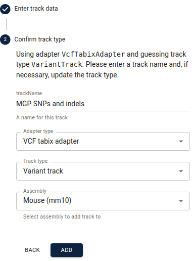
Go ahead and click the “Next” button. In the next step that appears, verify that all the information is correct and change the name of the track if you would like, e.g. to something more human-readable like "MGP SNPs and indels." Then click "Add". The new track will automatically open, and you can find the entry for it in the track selector under the automatically created "Session tracks" category.

Managing sessions

Now that we've customized the tracks in JBrowse a bit, how can we avoid having to do it again every time we want to view this data? JBrowse allows you to save and share its current state as a session. This includes any custom tracks that have been added, as well as the views and tracks that are currently open.

There are two main ways to save a session. The first one is JBrowse's automatic session saving. From the "File" menu, you can look under "Recent sessions…" and find your recent sessions. To find the session at a later time more easily, though, you can give the session a custom name. To do this, change the name of the session in the very top bar of JBrowse, between the "Help" menu and the "Share" button. When you come back to JBrowse later, you can find the session with this name from the "File -> Recent sessions…" menu.

The second way to save a session is to create a share link for it. You can do this by clicking the "Share" button in the top bar of JBrowse. It will then display a share link that can be sent to others to share your current session, or can be used as a type of bookmark to the session as it was when the link was created.

Exploring variants

For the next part of this tutorial, we're going to explore a missense mutation in the Msh3 gene. Make sure the original "NCBI RefSeq - RefSeq All" track and the "MGP SNPs and indels" track we just added are open. Then go to the location/search box, enter "msh3," and press “Enter.” This will navigate to the Msh3 gene. You may want to expand the RefSeq track to see all the transcripts. You can do this by clicking and dragging the bottom area of that track.

At this level you can't see the SNP track data, since there's too much data for that region and JBrowse doesn't want to risk overloading your computer. This is a good use case for the ruler bar zoom. In the area just above the top track, click and drag the area around the exon we want and click "Zoom to region" from the resulting menu.

In this tutorial we’ll have several times where we ask you to navigate to a certain location. When we do so, we’ll provide it in a table like the one below. The “Location” is what you can copy and paste into the location box to navigate to the region. We also provide a link to a session that is already at that location that you can use instead. Here’s an example for the location of the exon from above.

Location	Session
chr13:92,215,450..92,215,650	Link

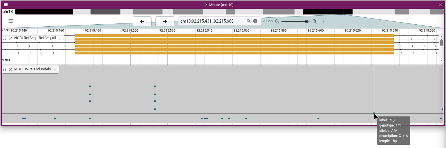
The SNP of interest is the one furthest to the right in the exon, labeled "C->A". Click on the SNP and explore the information about it on the details widget that pops up.

One thing to note is the sample table, which shows that the sample labeled "RF_J" (which is the RF/J mouse strain) is homozygous for the alternate allele, while all other samples are homozygous for the reference allele. If we want to know which of the other SNPs are present in which mouse strains, we can use another variant track display to see it at a glance. From the track menu (the three vertical dots next to the track label), select "Display types" and then "Multi-sample variant display (regular)". In this mode, every row is a sample, and each SNP is marked on the samples for which they exist. Zoom out and scroll around to get familiar with how this display shows the data.

When zoomed out further, you can see large-scale patterns in the data, and the track menu contains a lot of options for organizing and coloring the data to help you see what you’re looking for. We won’t focus on those today, but let us know if this would be of interest for a future tutorial.

Exploring short read DNA-seq alignments

As we saw above, the only strain with the missense variant was RF/J, so let’s inspect the reads for the variant call in that strain. To do this, we’ll add another track in the same way as above. The URL that you’ll enter is https://ftp.ebi.ac.uk/pub/databases/mousegenomes/REL-1905-CRAMs/RF_J.cram (and https://ftp.ebi.ac.uk/pub/databases/mousegenomes/REL-1905-CRAMs/RF_J.cram.crai if you want to enter the index file URL, although it’s again not necessary). Let’s name the track “MGP RF/J Illumina reads.”

You’ll notice in the second step that JBrowse correctly guesses the adapter type and track type for this file, which are different from the VCF file in the track we added above. Usually JBrowse can guess correctly, but in case of non-standard file names, you can select them from the drop-down boxes.

This is a CRAM file, which is a common file used to store alignments. You’ll also commonly see them stored in BAM files, which JBrowse can also use the same way as CRAM files.

Make sure you’re navigated back to the exon of interest from above. The reads track should now be open below the variants track.

Before we dive too deeply into exploring this track, we’re going to change it to make it a bit simpler and then come back to this version later. To do this we'll change the display type for the track by opening the track menu and choosing “Display types -> Pileup display.”

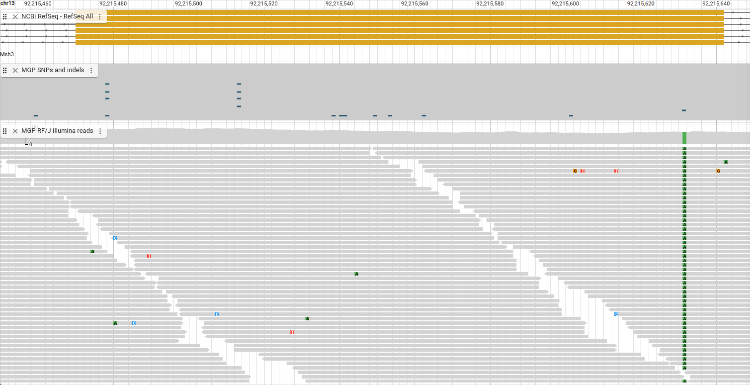
In this display, each box you see is a single read from the CRAM file. Spend a few minutes scrolling around, clicking on the reads, and seeing what information you can discover.

Now that you’ve had a chance to familiarize yourself with the track a bit, let’s explore what some parts of it mean. You may have noticed an arrow on one end of each box. That is the strand of the read. More information about what different things in the track mean is available by opening the track menu and selecting “Show legend.”

You also might notice that there are more reads than fit in the visible area in the track right now. You can scroll to see them, and you can also increase the height of the track by clicking and dragging the area at the bottom of the track. Another way to see more reads at a time is to decrease the height of the rectangles. To do this, open the track menu and select “Set feature height… -> Compact” (or Super-compact).

We can see the green boxes in our reads represent an “A,” and they are at the same position as the variant track, so that supports the “C -> A” SNP we find in that track.

Now that you’re more familiar with using the alignments tracks, let’s explore some more locations that illustrate more features of these tracks. All these examples are in this same gene, so you can zoom out and get an idea of where we are at any time. Before proceeding, though, go back to the “Normal” feature height so we can more easily see the track features.

Let’s look at a deletion next.

Location	Session
chr13:92,250,820..92,250,850	Link

The deletion shows up as gray bars in the reads with a number indicating the length of the deletion, and they align with a deletion in the “MGP SNPs and indels” track.

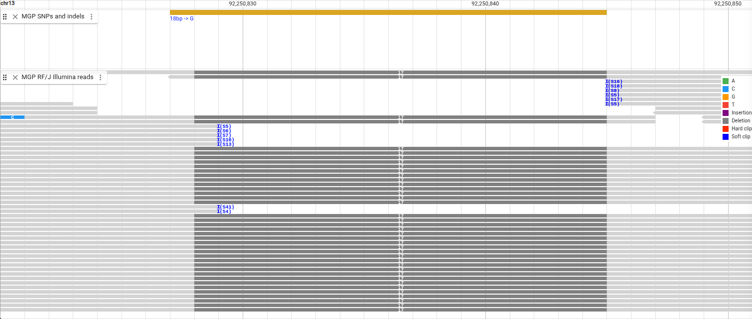
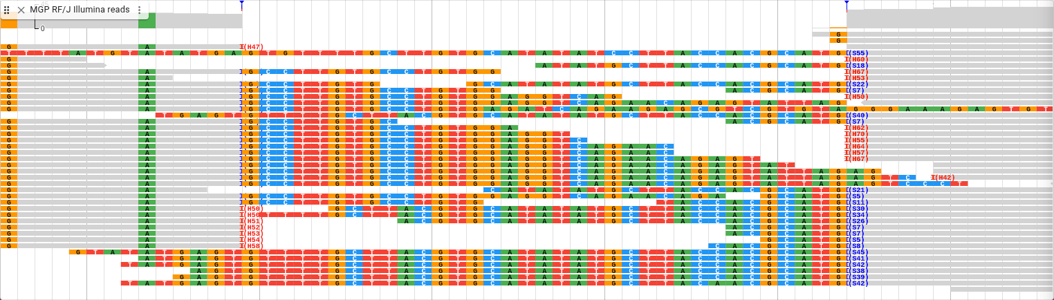
We can also see some blue “I”s indicating that the reads have soft clipping. We are able to view the soft clipped bases by selecting “Show -> Show soft clipping” in the track menu. We can also group all the reads with deletions next to each other by sorting them.

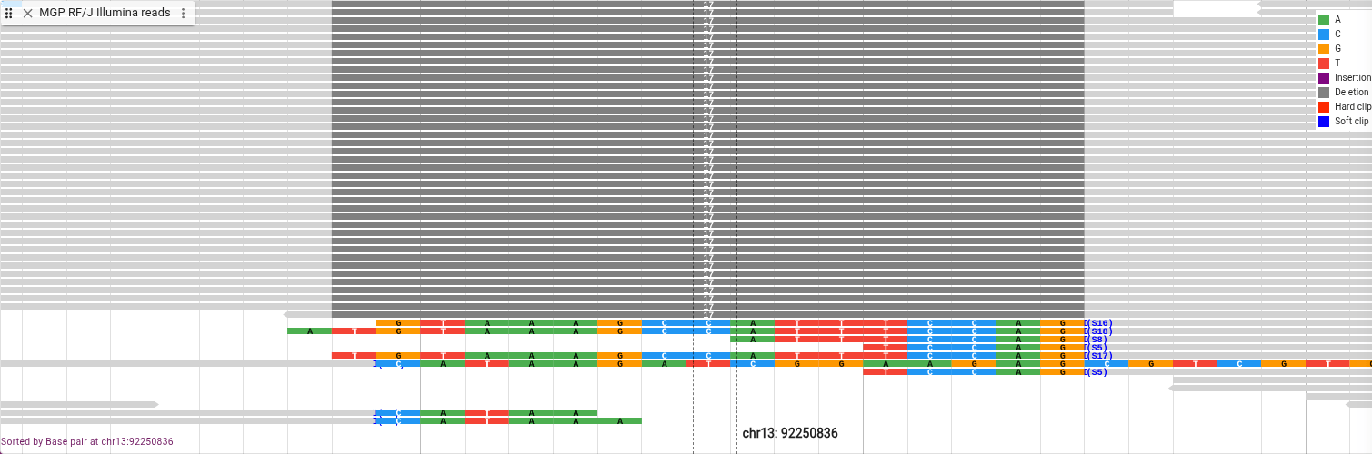
Sorting is based on the reads at the center of the view. To better see where the center is, open the view menu from the button with three horizontal lines (sometimes called a hamburger menu) in the top left of the view. From that menu, select “Show… -> Show center line.” This creates a set of dotted lines showing where the center of the view falls. Align that to the center of the deletion and from the track menu select “Sort by… -> Base pair.”

Now we’ll look at an insertion.

Location	Session
chr13:92,252,835..92,252,865	Link

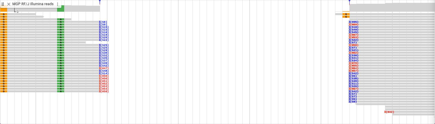
Insertions show up as a purple box that is between bases with the length of the insertion printed inside it. Shown below is this insertion with the soft clipping turned back off and the sorting cleared.

Before we go to the next location, we are going to change the display type again. From the track menu, select “Display types -> SNPCoverage display” and navigate to the next location.

Location	Session
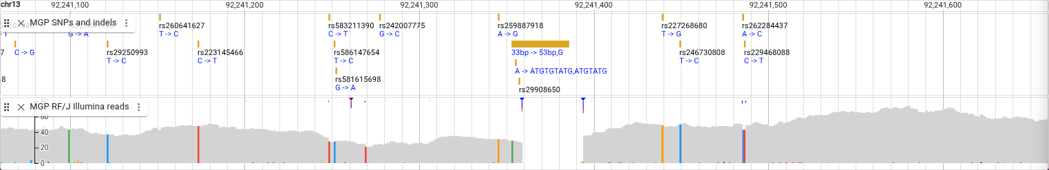
chr13:92,241,060..92,241,660	Link

This display shows a coverage plot, so instead of showing each read, it shades the plot based on how many reads are present at each base pair. You can see on the left the scale of the plot, and you can get the exact value of the depth by hovering over a location in the plot. You can see here that there is a deletion, illustrated by the coverage plot showing a region with zero depth.

We’ve now seen the Pileup and SNPCoverage displays. The default display that we will go back to now is actually a combination of those two displays. From the track menu, select “Display types -> Alignments display (combination)”

All the settings we changed while using the Pileup Display are now in a sub-menu called “Pileup settings” in the track menu. You also can replace the lower Pileup display with other displays that we will explore shortly.

First, though, let’s zoom in on the deletion we saw above.

Location	Session
chr13:92,241,345..92,241,405	Link

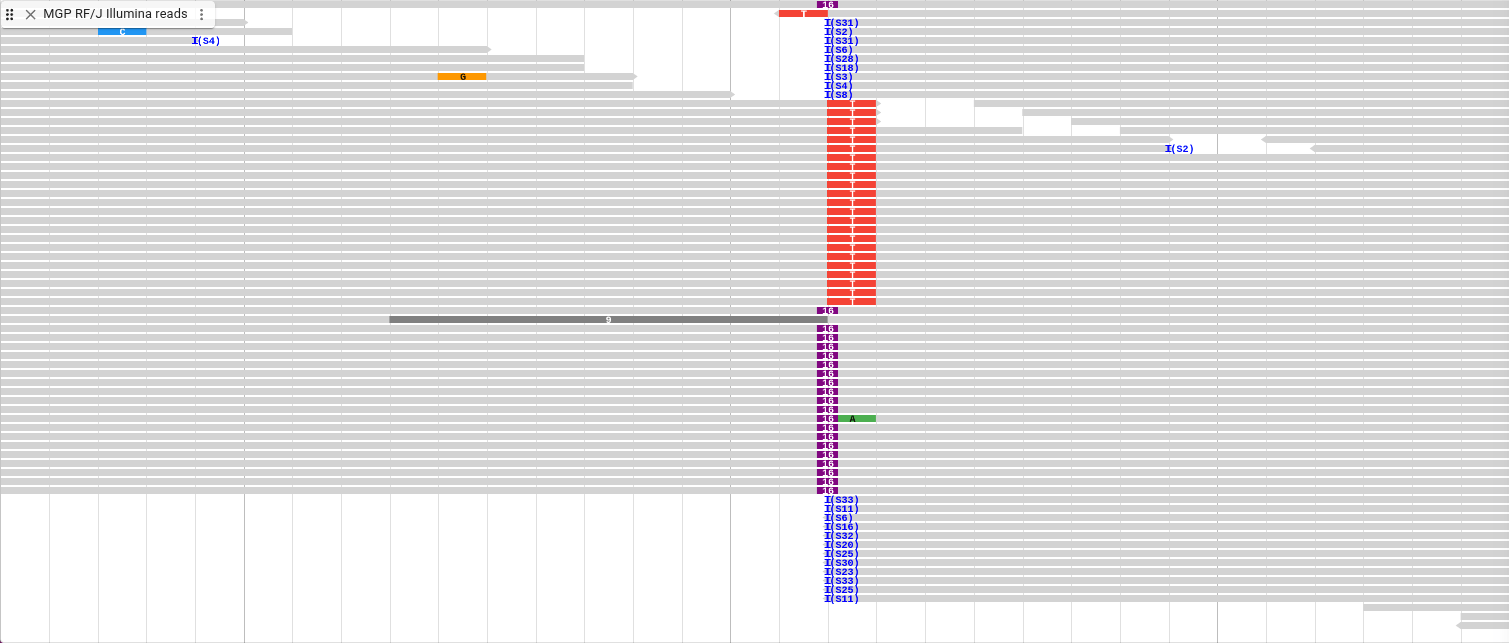
You can see that for this deletion, there are no reads that span it, so the area where the deletion is located is empty. You can still see the soft clipping indicators, though, as well as some hard clipping indicators.

Let’s show the soft clipping again. You can see that for the hard clipping indicators, unlike the soft clipping, the clipped sequence is not stored in the file, so they cannot be viewed.

We’re now going to try a different type of display. In the track menu, select “Display types -> Read arc display” and also “Show legend.” Now navigate to this location.

Location	Session
chr13:92,267,260..92,273,760	Link

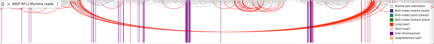
These arcs are connecting the two ends of these paired-end short reads. Any reads with their mate on another chromosome are represented by a purple vertical line. Read pairs where the separating distance is on the same chromosome but long (over three standard deviations above the average) are shown with red arcs. As we can see, there is group of reads in the same region that are all separated by a long distance from their mates.

How many of these reads have long inserts, compared to the total number of reads? To find out, we’ll look at another display type. In the track menu, select “Display types -> Linked reads display,” then “Show legend,” then also “Set feature height.. -> Compact”

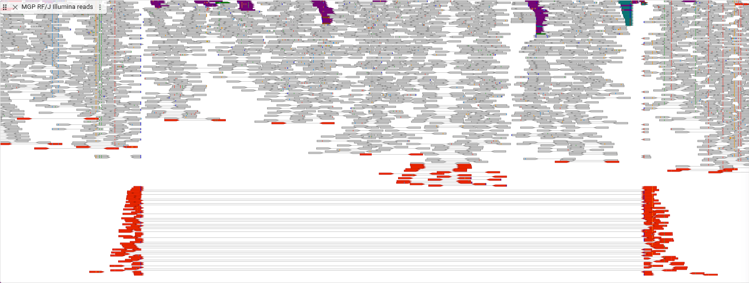
In this display, the lined reads are drawn on the same row and are connected by a line, allowing you to see how many of these types of reads there are.

Exploring long read RNA-seq alignments

Up until now we’ve been looking at Illumina short-read DNA sequencing data. To illustrate a few more features of the alignments tracks, let’s look at some PacBio long-read RNA sequencing data.

We’ll add a new track called “PacBio RNA-seq Brain,” and the URL is https://ftp.ebi.ac.uk/pub/databases/havana/ngs_havana/CLS/updated_master_table/mouse/pacBioSII-Cshl-CapTrap_Mv2_0+_Brain01Rep1.bam. (Index is https://ftp.ebi.ac.uk/pub/databases/havana/ngs_havana/CLS/updated_master_table/mouse/pacBioSII-Cshl-CapTrap_Mv2_0+_Brain01Rep1.bam.bai, but is again optional.)

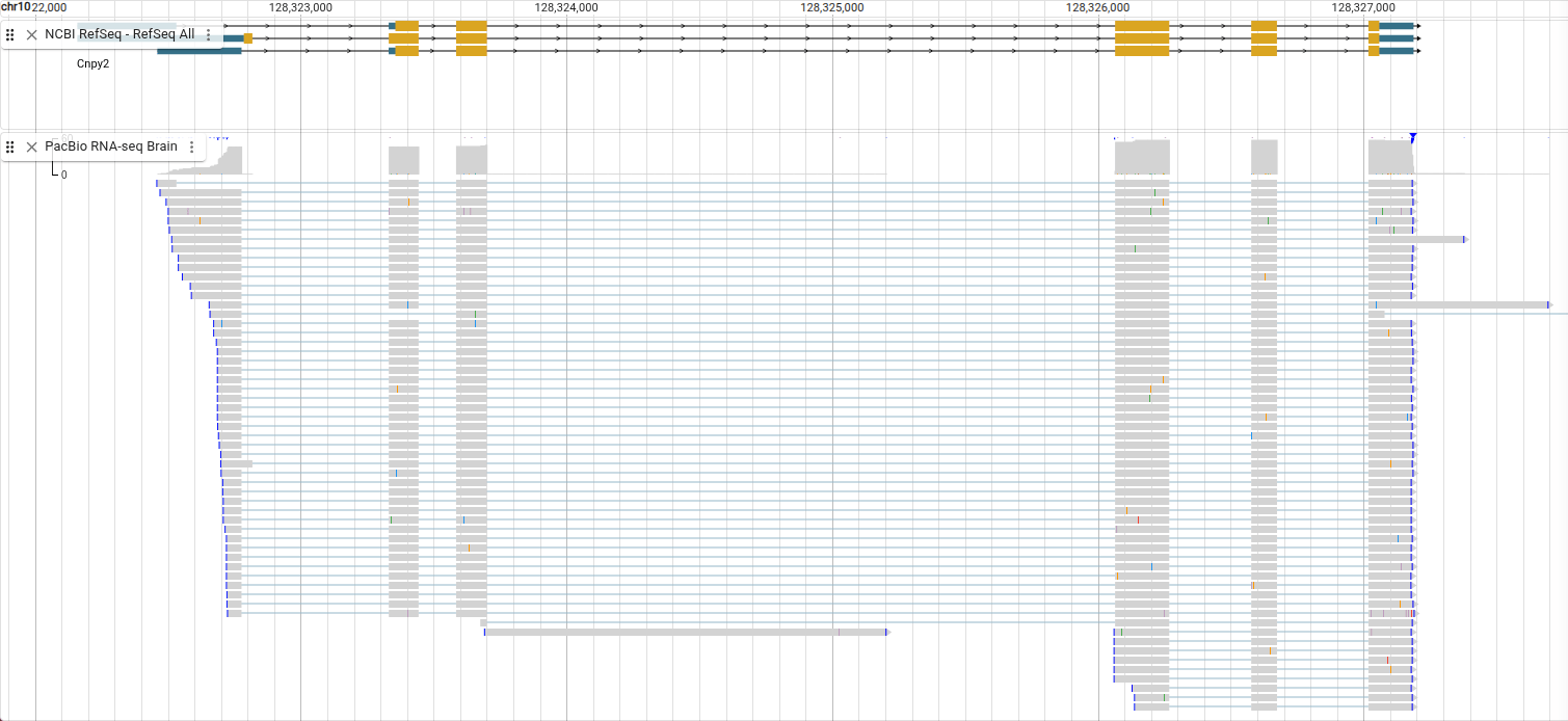
You can close all the other tracks except this one and the “NCBI RefSeq - RefSeq All” track. Then navigate to the Cnpy2 gene. In addition to the usual options below, you can also get there by entering "Cnpy2" in the location box.

Location	Session
chr10:128,321,870..128,327,770	Link

In RNA-seq reads like these, a single read can be split across many locations, and the locations are connected by lines. As you can see, the areas where the reads align match the exons in the Cnpy2 gene.

Showing soft clipping with RNA-seq reads also allows you to see something else about the reads. Select “Pileup settings -> Show -> Show soft clipping” from the track menu.

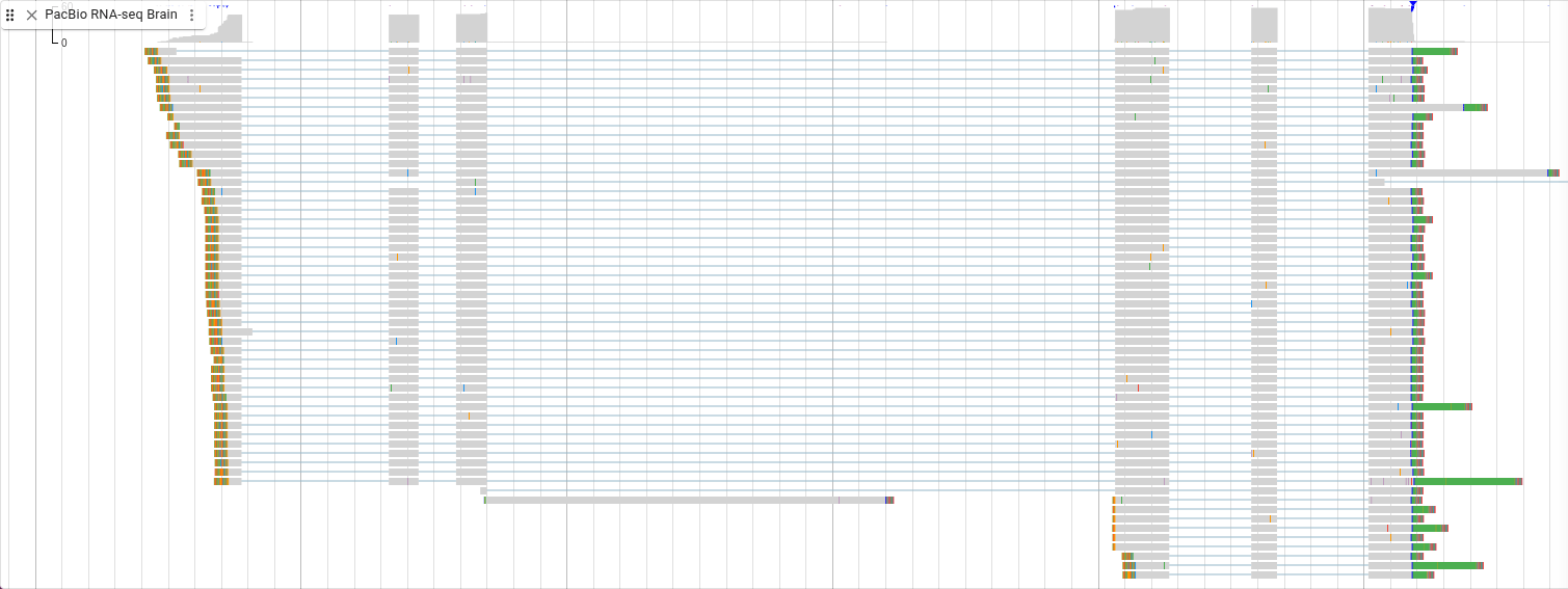
On the right side of these reads you can see green bars. Remember that green is the color for the base “A.” These are the poly(A) tails of the mRNA.